Chapter 1 Seawater properties

1.1 gravitational acceleration

Fig. 1.1 shows the influence of latitude and pressure \(p\) on gravitational acceleration \(g\).

library(gsw)
lats <- seq(0, 90, l=100)
p <- seq(0, 6000, l=100)
g <- outer(lats, p, function(x,y) gsw::gsw_grav(latitude=x, p=y))
g_rel_to_981 <- g/9.81*100 - 100
par(mfrow=c(1, 2), mar=c(5, 6, 4, 2))
plot(lats, p, t="n", xaxt="n", yaxt="n", ylim=c(max(p), min(p)),
     xlab="Latitude [°]", ylab=NA,
     xaxs="i", yaxs="i")
axis(1, at=pretty(lats, n=10))
axis(2, at=pretty(p, n=10), las=2)
mtext("Depth [dbar]", side=2, line=4)
abline(v=45, col="gray")
contour(lats, p, g, levels=pretty(g, n=10), labcex=1, add=T)
contour(lats, p, g, levels=9.81, col="red", add=T, drawlabels=F)
plot(lats, p, t="n", xaxt="n", yaxt="n", ylim=c(max(p), min(p)),
     xlab="Latitude [°]", ylab=NA,
     xaxs="i", yaxs="i")
axis(1, at=pretty(lats, n=10))
axis(2, at=pretty(p, n=10), las=2)
mtext("Depth [dbar]", side=2, line=4)
abline(v=45, col="gray")
contour(lats, p, g_rel_to_981, levels=pretty(g_rel_to_981, n=10), 
        labels=pretty(g_rel_to_981, n=10), labcex=1, add=T)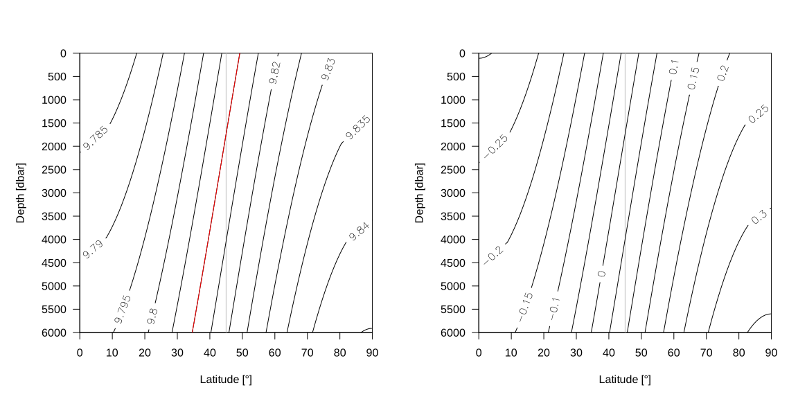

Fig. 1.1: Gravitational acceleration \(g\) as a function of latitude and pressure \(p\) (in m s\(^{-2}\), left) and relative to 9.81 m s\(^{-2}\) (in %, right).

1.2 heat capacity of seawater

Fig. 1.2 shows the influence of in-situ temperature \(t\) and absolute salinity \(S_A\) on heat capacity of seawater \(c_\text{p}\) at different pressure \(p\) levels.

cp0 <- 3991.86795711963 # J/(kg K); from GSW-R/src/gsw_internal_const.h
p <- c(0, 1000, 2000, 4000)
SA <- seq(0, 40, l=100)
t_insitu <- seq(-2, 30, l=100)
cps <- array(NA, dim=c(length(SA), length(SA), length(p)))
for (i in 1:length(p)) {
    cps[,,i] <- outer(SA, t_insitu, function(x,y) gsw::gsw_cp_t_exact(SA=x, t=y, p=p[i]))
}
zlim <- range(cps, na.rm=T)
zat <- pretty(zlim, n=15)
cps_rel <- cps/cp0*100 - 100
zlim_rel <- range(cps_rel, na.rm=T)
zat_rel <- pretty(zlim_rel, n=15)
par(mfrow=c(length(p), 2), mar=c(5, 6, 4, 2))
xat <- pretty(t_insitu, n=15)
yat <- pretty(SA, n=15)
for (i in 1:length(p)) { 
    # absolute plots
    plot(t_insitu, SA, t="n", xaxt="n", yaxt="n",
         xlab="In-situ temperature [°C]", ylab=NA,
         xaxs="i", yaxs="i")
    abline(v=xat, col="gray", lwd=0.5)
    abline(h=yat, col="gray", lwd=0.5)
    axis(1, at=xat)
    axis(2, at=yat, las=2)
    mtext("Absolute salinity [g/kg]", side=2, line=4)
    contour(t_insitu, SA, cps[,,i], levels=zat, labcex=1, add=T)
    contour(t_insitu, SA, cps[,,i], levels=cp0, labcex=1, col="red", add=T)
    legend("topright", paste0(p[i], " dbar"), lty=NA, pch=NA, lwd=NA, bty="n")
    # relative plots
    plot(t_insitu, SA, t="n", xaxt="n", yaxt="n",
         xlab="In-situ temperature [°C]", ylab=NA,
         xaxs="i", yaxs="i")
    abline(v=xat, col="gray", lwd=0.5)
    abline(h=yat, col="gray", lwd=0.5)
    axis(1, at=xat)
    axis(2, at=yat, las=2)
    mtext("Absolute salinity [g/kg]", side=2, line=4)
    contour(t_insitu, SA, cps_rel[,,i], levels=zat_rel, 
            labels=zat_rel, labcex=1, add=T)
    legend("topright", paste0(p[i], " dbar"), lty=NA, pch=NA, lwd=NA, bty="n")
}

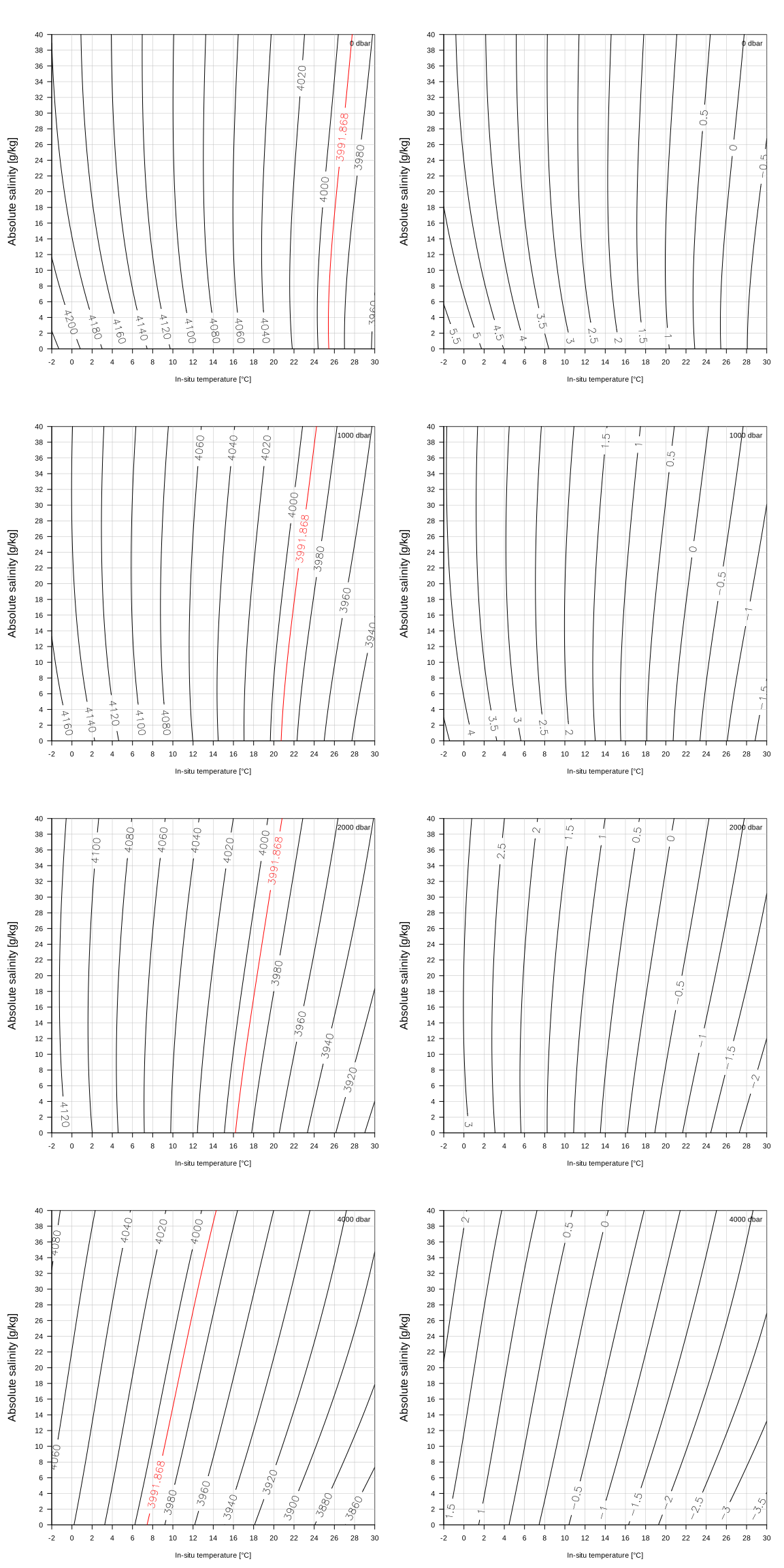
Fig. 1.2: Heat capacity of seawater \(c_p\) as a function of in-situ temperature \(t\) and absolute salinity \(S_A\) (in m\(^2\) s\(^{-2}\) K\(^{-1}\), left) and relative to \(c_{p,0}\) = 3991.86795711963 m\(^2\) s\(^{-2}\) K\(^{-1}\) (in %, right) at different depths.

1.3 speed of sound

Fig. 1.3 shows the influence of in-situ temperature \(t\) and absolute salinity \(S_A\) on speed of sound \(c\) at different pressure \(p\) levels.

p <- c(0, 1000, 2000, 4000)
SA <- seq(0, 40, l=100)
t_insitu <- seq(-2, 30, l=100)
soss <- array(NA, dim=c(length(SA), length(SA), length(p)))
for (i in 1:length(p)) {
    soss[,,i] <- outer(SA, t_insitu, function(x,y) gsw::gsw_sound_speed_t_exact(SA=x, t=y, p=p[i]))
}
zlim <- range(soss, na.rm=T)
zat <- pretty(zlim, n=15)
sos0 <- mean(soss, na.rm=T)
soss_rel <- soss/sos0*100 - 100
zlim_rel <- range(soss_rel, na.rm=T)
zat_rel <- pretty(zlim_rel, n=15)
par(mfrow=c(length(p), 2), mar=c(5, 6, 4, 2))
xat <- pretty(t_insitu, n=15)
yat <- pretty(SA, n=15)
for (i in 1:length(p)) { 
    # absolute plots
    plot(t_insitu, SA, t="n", xaxt="n", yaxt="n",
         xlab="In-situ temperature [°C]", ylab=NA,
         xaxs="i", yaxs="i")
    abline(v=xat, col="gray", lwd=0.5)
    abline(h=yat, col="gray", lwd=0.5)
    axis(1, at=xat)
    axis(2, at=yat, las=2)
    mtext("Absolute salinity [g/kg]", side=2, line=4)
    contour(t_insitu, SA, soss[,,i], levels=zat, labcex=1, add=T)
    contour(t_insitu, SA, soss[,,i], levels=sos0, labcex=1, col="red", add=T)
    legend("topright", paste0(p[i], " dbar"), lty=NA, pch=NA, lwd=NA, bty="n")
    # relative plots
    plot(t_insitu, SA, t="n", xaxt="n", yaxt="n",
         xlab="In-situ temperature [°C]", ylab=NA,
         xaxs="i", yaxs="i")
    abline(v=xat, col="gray", lwd=0.5)
    abline(h=yat, col="gray", lwd=0.5)
    axis(1, at=xat)
    axis(2, at=yat, las=2)
    mtext("Absolute salinity [g/kg]", side=2, line=4)
    contour(t_insitu, SA, soss_rel[,,i], levels=zat_rel, 
            labels=zat_rel, labcex=1, add=T)
    legend("topright", paste0(p[i], " dbar"), lty=NA, pch=NA, lwd=NA, bty="n")
}

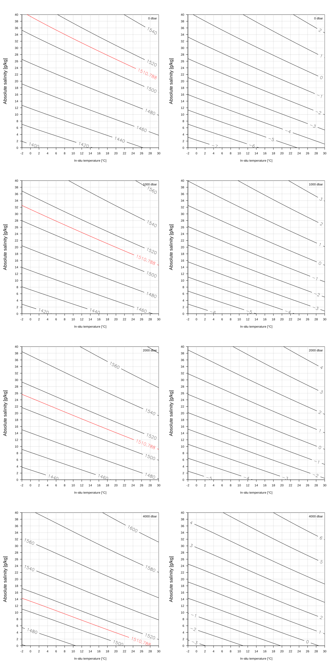
Fig. 1.3: Speed of sound \(c\) as a function of in-situ temperature \(t\) and absolute salinity \(S_A\) (in m s\(^{-1}\), left) and relative to \(c_0\) = 1510 m s\(^{-1}\) (in %, right) at different depths.